8. 2D Example
The nonstandard (NS) FDTD algorithm provides much higher accuracy than standard (S) FDTD one for the cylindrical Mie scattering.
Here we introduce Mie solutions in the TM and TE modes and compare numerical solutions of S- and NS-FDTD algorithms with the analytic.
Cylindrical Mie Scattering
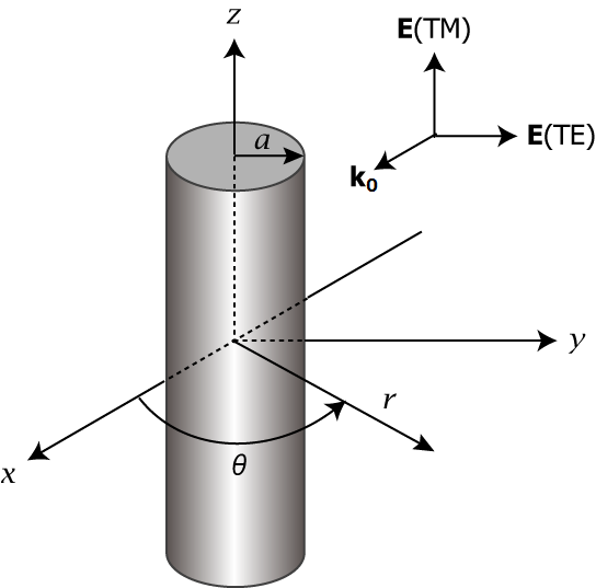
Fig. 1. Infinite plane wave impinging on an infinite dielectric cylinder (a = radius, k0 = wave vector in vacuum).
TH and TE polarizations are shown. Wave propagates along +x axis.
Maxwell's equations can be reduced to the Helmholtz equation for Ez,
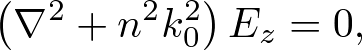 . . . (1)
where n is the refractive index and k0 is the wavenumber in vacuum.
This Helmholtz equation for an infinite cylinder shown in Fig. 1 is solved by Mie theory [1].
In the TM mode, Ez is independent of z so Ez = Ez(x, y).
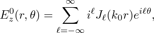
Outside the cylinder, Ez is the sum of the incident field Ez0 = eik0x
and the outgoing scattered field Ezs. Taking (x, y) = r(cosθ, sinθ),
Ezs can be expanded in the form,
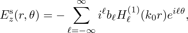 . . . (2)
where Hl(1) is the Hankel function of the first kind and the bl is the expansion coefficient to be determined.
The electric field inside the cylinder, Ezi, can be expanded in the form,
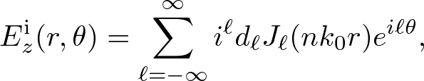 . . . (3)
where Jl is the Bessel function of the first kind and dl is the expansion coefficient.
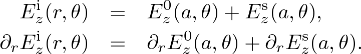
The expansion coefficients, bl and dl, are determined by the physical conditions that
both Ez and its derivative ∂r must be continuous on the cylinder boundary. Using the fact that
 . . . (4)
we obtain
 . . . (5)
Using the identity Z'l(x) = Zl-1(x) - (l/x)Zl(x) where Zl = Jl and Hl(1),
we can determine the expansion coefficients. Abbreviating x = k0a, we find
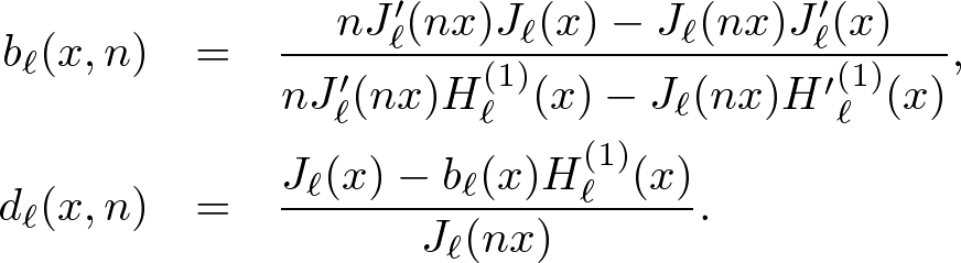 . . . (6)
In the TE mode, the incident polarization is defined by Er0 = eik0xsinθ and
Eθ0 = eik0xcosθ. Similarly, we obtain the outgoing scattered field,
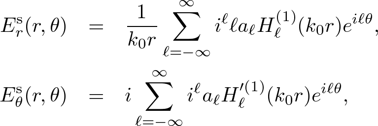 . . . (7)
and the electric field inside the cylinder is given by
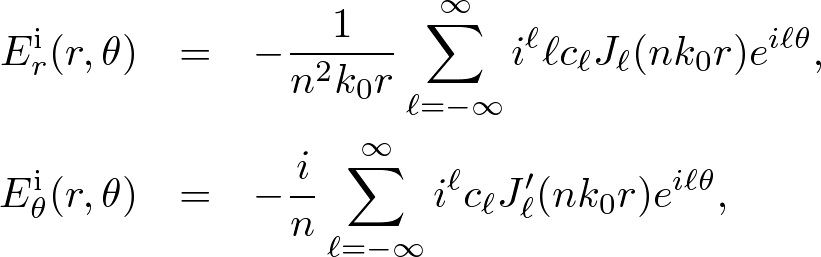 . . . (8)
where
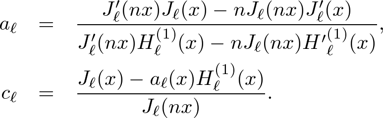 . . . (9)
The transform from polar coordinates to Cartesian ones is given by
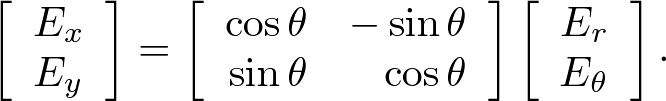 . . . (10) Example Simulation
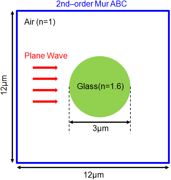
Figure 2 is an example Mie scattering in the TM mode. The computational domain is terminated by 2nd-order Mur ABC.
Inside infinite cylinder consists of optical glass and outside is air.
Fig. 2. Example simulation of Mie scattering in the TM mode. Computational domain is 12μm×12μm and is terminated by 2nd-order Mur ABCs.
Inside infinite cylinder consists of optical glass and outside is air.
Simulation parameters are listed in Table 1.
Table. 1. Simulation parameters.
| Source wavelength λ |
Grid spaceing h |
| 1550nm |
150nm |
Since Maxwell's equations are equivalent to the wave equation in the TM mode, let us solve latter.
Because the NS-FDTD program can be easily reduced to the S-FDTD one, let us program the NS-FDTD simulation.
As below, we separate the program into FDTD computation and visualization parts.
FDTD Computation
We describe the two-dimensional NS-FDTD simulation class based on scattered field formulation in Source 1.
Source. 1. Two-dimensional FDTD calculation class. [Download Source 1]
// One-dimensional FDTD simulation
class FDTD2D {
private:
    int     Nx, Ny;         // grid size
    int     num_elements;   // number of grid points
    double  v;              // wave speed
    double  h;              // grid spacing
    double  dt;             // time interval
    double  lambda;         // wavelength
    double  k;              // wavenumber
    double  omega;          // angular frequency
    double  radius;         // cylinder radius
    double* psi_next;       // next field
    double* psi_current;    // current field
    double* psi_previous;   // previous field
    double* u;              // coefficient matrix
    double* n;              // refractive index
    double* gamma1;         // gamma coefficient for NS-FDTD
    double  t;              // simulation time

public:
    // Initialization
    void Initialize( void )
    {
        Nx = Ny = 12000/150;      // grid size
        num_elements = Nx * Ny;   // number of grid points
        h      = 1;               // grid spacing
        dt     = 1;               // time interval
        v      = 0.7;             // wave speed
        lambda = 1550 / 150;      // wavelength
        k      = 2*M_PI/lambda;   // wavenumber
        omega  = v * k;           // angular frequency
        radius = 1500 / 150;      // cylinder radius

        // Get memory
        psi_next     = new double [num_elements];
        psi_current  = new double [num_elements];
        psi_previous = new double [num_elements];
        u            = new double [num_elements];
        n            = new double [num_elements];
        gamma1       = new double [num_elements];

        // Set init field
        for ( int i=0; i<num_elements; i++ ) {
            // wave field
            psi_next[i] = psi_current[i] = psi_previous[i] = 0;
        }

        // Set media distribution
        FuzzyModel();
        // Set u and gamma1
        SetCoefficients();
    }

    // Finalize
    void Finalize( void )
    {
        // Release memory
        delete [] psi_next;
        delete [] psi_current;
        delete [] psi_previous;
        delete [] u;
        delete [] n;
        delete [] gamma1;
    }

    // Get index
    int idx( int i, int j )
    {
        return ( i*Ny + j );
    }

    // Set scatterer
    bool IsInCircle( double x, double y, double r )
    {
        if ( x*x + y*y <= r*r ) return true;
        else return false;
    }

    // Set Permittivity
    void FuzzyModel()
    {
        // glass refractive index
        double n_glass = 1.6;

        for ( int i=0; i<Nx; i++ ) {
            for ( int j=0; j<Ny; j++ ) {
                // Get index
                int id = idx( i, j );

                // Get center
                double cx = (Nx-1) / 2.0;
                double cy = (Ny-1) / 2.0;
                // Get position
                double x = i - cx;
                double y = j - cy;

                // subgrid size
                int subN = 20;
                // Get areas
                double area;
                for ( int p=0; p<subN; p++ ) {
                    for ( int q=0; q<subN; q++ ) {
                        // Get shifted position
                        double sx = x - 0.5 + p/(double)(subN-1);
                        double sy = y - 0.5 + q/(double)(subN-1);
                        if ( IsInCircle( sx, sy, radius ) ) {
                            area += 1.0;
                        }
                    }
                }
                area /= (double)(subN*subN);

                // Set permittivity by Fuzzy model
                n[id] = sqrt( n_glass*n_glass*area + (1.0-area) );
            }
        }
    }

    // Set u and gamma1
    void SetCoefficients()
    {
        for ( int i=0; i<Nx; i++ ) {
            for ( int j=0; j<Ny; j++ ) {
                // Get index
                int id = idx( i, j );
                // Set u
                u[id] = sin(omega*dt/2) / sin(k*n[id]*h/2);
                // Set gamma1
                gamma1[id] = 1.0/6.0 + (k*n[id])*(k*n[id])*h*h*(
                    1.0/180.0 - (k*n[id])*(k*n[id])*h*h/23040.0 );
            }
        }
    }

    // Nonstandard Mur ABC
    void nsMurABC( int i, int j )
    {
        double u1 = tan(omega*dt/2) / tan(k*h/2);
        double th = M_PI / 3;
        double u2 = 2*sin(omega*dt/2)*sin(omega*dt/2)
                  * ( 1-tan(k*h*cos(th)/2)/tan(k*h/2) )
                  / (sin(k*h*sin(th)/2)*sin(k*h*sin(th)/2));

        // left
        if ( i==0 ) {
            psi_next[idx(0,j)] = - psi_previous[idx(1,j)]
            + (u1-1)/(u1+1)*( psi_next[idx(1,j)]+psi_previous[idx(0,j)] )
            + 2/(u1+1)*( psi_current[idx(1,j)] + psi_current[idx(0,j)] )
            + 0.5*u2*u2/(u1+1)*( psi_current[idx(1,j+1)]
            + psi_current[idx(1,j-1)] - 2*psi_current[idx(1,j)]
            + psi_current[idx(0,j+1)] + psi_current[idx(0,j-1)]
            - 2*psi_current[idx(0,j)] );
        }
        // right
        if ( i==Nx-1 ) {
            psi_next[idx(Nx-1,j)] = - psi_previous[idx(Nx-2,j)]
            + (u1-1)/(u1+1)*( psi_next[idx(Nx-2,j)]+psi_previous[idx(Nx-1,j)] )
            + 2/(u1+1)*( psi_current[idx(Nx-2,j)] + psi_current[idx(Nx-1,j)] )
            + 0.5*u2*u2/(u1+1)*( psi_current[idx(Nx-2,j+1)]
            + psi_current[idx(Nx-2,j-1)] - 2*psi_current[idx(Nx-2,j)]
            + psi_current[idx(Nx-1,j+1)] + psi_current[idx(Nx-1,j-1)]
            - 2*psi_current[idx(Nx-1,j)] );
        }
        // bottom
        if ( j==0 ) {
            psi_next[idx(i,0)] = - psi_previous[idx(i,1)]
            + (u1-1)/(u1+1)*( psi_next[idx(i,1)]+psi_previous[idx(i,0)] )
            + 2/(u1+1)*( psi_current[idx(i,1)] + psi_current[idx(i,0)] )
            + 0.5*u2*u2/(u1+1)*( psi_current[idx(i+1,1)]
            + psi_current[idx(i-1,1)] - 2*psi_current[idx(i,1)]
            + psi_current[idx(i+1,0)] + psi_current[idx(i-1,0)]
            - 2*psi_current[idx(i,0)] );
        }
        // top
        if ( j==Ny-1 ) {
            psi_next[idx(i,Ny-1)] = - psi_previous[idx(i,Ny-2)]
            + (u1-1)/(u1+1)*( psi_next[idx(i,Ny-2)]+psi_previous[idx(i,Ny-1)] )
            + 2/(u1+1)*( psi_current[idx(i,Ny-2)] + psi_current[idx(i,Ny-1)] )
            + 0.5*u2*u2/(u1+1)*( psi_current[idx(i+1,Ny-2)]
            + psi_current[idx(i-1,Ny-2)] - 2*psi_current[idx(i,Ny-2)]
            + psi_current[idx(i+1,Ny-1)] + psi_current[idx(i-1,Ny-1)]
            - 2*psi_current[idx(i,Ny-1)] );
        }
    }

    // Update field
    void Update( void )
    {
        // Shift memory target
        double* temp = psi_previous;
        psi_previous = psi_current;
        psi_current  = psi_next;
        psi_next     = temp;

        // Update field
        for ( int i=1; i<Nx-1; i++ ) {
            for ( int j=1; j<Ny-1; j++ ) {
                // Get index
                int id = idx( i, j );
                // additional difference
                double dx2dy2 =
                    +   psi_current[idx(i-1,j+1)] - 2*psi_current[idx(i  ,j+1)]
                    +   psi_current[idx(i+1,j+1)] - 2*psi_current[idx(i-1,j  )]
                    + 4*psi_current[idx(i  ,j  )] - 2*psi_current[idx(i+1,j  )]
                    +   psi_current[idx(i-1,j-1)] - 2*psi_current[idx(i  ,j-1)]
                    +   psi_current[idx(i+1,j-1)];
                // NS-FDTD
                psi_next[id] = - psi_previous[id] + 2*psi_current[id]
                    + u[id]*u[id]*( psi_current[idx(i+1,j)]
                    + psi_current[idx(i,j+1)] + psi_current[idx(i-1,j)]
                    + psi_current[idx(i,j-1)] - 4*psi_current[id]
                    +gamma1[id]*dx2dy2 );

                // Add incident field
                psi_next[id] += ( 1/(n[id]*n[id]) - 1 )
                    * ( Source(k,i,omega,t+dt)
                    - 2*Source(k,i,omega,t) + Source(k,i,omega,t-dt) );
            }
        }

        // Set boundary condition
        for ( int j=1; j<Ny-1; j++ ) {
            nsMurABC(0,j);
            nsMurABC(Nx-1,j);
        }
        for ( int i=1; i<Nx-1; i++ ) {
            nsMurABC(i,0);
            nsMurABC(i,Ny-1);
        }

        // Update t
        t += dt;
    }

    // Incident field
    double Source( double k, double x, double omega, double t )
    {
        // damping coefficient
        double w = 1.0 - exp(-pow(0.01*t,2));
        return w * sin( k*x - omega*t );
    }

    // Get number of grid points
    int GetNx()
    {
        return Nx;
    }
    int GetNy()
    {
        return Ny;
    }

    // Get current field value
    double GetValue( int i, int j )
    {
        return psi_current[idx(i,j)];
    }

    // Get intensity
    double GetIntensity( int i, int j )
    {
        // Get index
        int id = idx( i, j );

        // Get field values
        double v0 = psi_next[id];
        double v1 = psi_current[id];
        double v2 = psi_previous[id];

        // Calculate time difference
        double a = ( v0-v2 ) / ( 2*sin(omega*dt) );
        double b = ( v0+v2-2.0*v1 ) / ( 4.0*sin(omega*dt/2)*sin(omega*dt/2) );

        // Return intensity
        return a*a + b*b;
    }
};
|
The functions are
- Initialize:
(1) Define simulation parameters; (2) Allocate field and coefficient memoris; (3) Initialize field and set coefficients.
- Finalize:
Release memories.
- idx:
Map 2D index on 1D one.
- IsInCircle:
Determine inside or outsider cylinder.
- FuzzyModel:
Set refractive index based on the fuzzy model.
- SetCoefficients:
Set NS-FDTD coefficients.
- nsMurABC:
Set the nonstandard 2nd-order Mur ABC at (1) left, (2) right, (3) bottom, and (4) top boundaries.
- Update:
Calculate next time step. (1) Shift memory target; (2) Update field using the NS-FDTD algorithm. (3) Set nonstandard Mur ABC; (4) Update time step.
- GetNumNx, GetNumNy:
Return the number of grid points.
- GetValue:
Return calculated field value indexed by id.
- GetIntensity:
Return intensity indexed by id.
OpenGL Visualization
Let us program an interactive calculation using the GLUT.
Source 2 is a main program includes GLUT visualization.
Source. 2. GLUT visualization of FDTD simulation. [Download Source 2]
// Include header files
#include "fdtd2d.h"
#include "glut.h"

// FDTD2D class
FDTD2D fdtd;

// Keyboard event
void keyboard( unsigned char key, int x, int y )
{
    switch ( key ) {
        // pushed 't' key
        case 't':
            fdtd.Update();         // Update field
            glutPostRedisplay();   // Redisplay
            break;
        default:
            break;
    }
}

// Transform from value to color
void Val2Col( double v, double* r, double* g, double* b )
{
    // Normalize value
    float nv = max( 0.0, min( 1.0, abs(v) ) );

    // Get color
    if      ( v >= 0.75 ) { *r = 1.0; *g = 4.0*(1.0-nv); *b = 0.0; }
    else if ( v >= 0.50 ) { *r = 4.0*(nv-0.5); *g = 1.0; *b = 0.0; }
    else if ( v >= 0.25 ) { *r = 0.0; *g = 1.0; *b = 4.0*(0.5-nv); }
    else                  { *r = 0.0; *g = 4.0*nv;       *b = 1.0; }
}

// Redisplay event
void display( void )
{
    // Clear background
    glClear( GL_COLOR_BUFFER_BIT );

    // Begin to draw points
    glBegin( GL_POINTS );

    // Draw distribution
    double r, g, b;
    for ( int i=0; i<fdtd.GetNx(); i++ ) {
        for ( int j=0; j<fdtd.GetNy(); j++ ) {
            // Get intensity
            double intensity = fdtd.GetIntensity( i, j );
            // point coordinates
            double x = -1.0 + 2*(i)/(double)(fdtd.GetNx()-1);
            double y = -1.0 + 2*(j)/(double)(fdtd.GetNy()-1);
            // Coloring
            Val2Col( intensity, &r, &g, &b );
            glColor4d( r, g, b, 1 );
            // Draw point
            glVertex2d( x, y );
        }
    }

    // End to draw lines
    glEnd();

    // Update view
    glFlush();
}

// Main function
int main( int argc, char** argv )
{
    // Initialize
    fdtd.Initialize();

    // Initialize GL
    glutInitWindowPosition( 50, 50 );     // window position
    glutInitWindowSize( 400, 400 );       // window size
    glutInitDisplayMode( GLUT_SINGLE );   // display mode
    glutInit( &argc, argv );              // Initialize GLUT
    glutCreateWindow( "FDTD" );           // Create window
    glutKeyboardFunc( keyboard );         // Register keyboard events
    glutDisplayFunc( display );           // Register display events
    glPointSize( 8 );                     // point size

    // GL loop
    glutMainLoop();

    // Finalize
    fdtd.Finalize();

    return 0;
}
|
Here we show rough flow of functions,
- keyboard:
Reply to keyboard events, where for t-key: (1) Update wave field; (2) Post a display event.
- Val2Col:
Intensity coloring (blue < green < red).
- display:
Draw figures: (1) Clear canvas; (2) Draw colored intensity distribution; (3) Display the figure.
- main:
(1) Initialize FDTD class; (2) Initialize OpenGL using GLUT library; (3) Start main loop. This loop is held up processing events until the window is closed; (4) Finalize FDTD class.
Figures 3 show the FDTD simulation results. Figure (a), (b), (c) are analytic, S-FDTD, NS-FDTD results, respectively.
The NS-FDTD algorithm provides remarkably higher accuracy than the FDTD algorithm.
.jpg) |
.gif) |
.gif) |
| (a) Analytic |
(b) Standard FDTD |
(c) Nonstandard FDTD |
Fig. 3. Intensity distributions of Mie scattering simulation: (a) Analytic; (b) Standard FDTD; and (c) Nonstandard FDTD.
Bibliography:
[1] P. W. Barber, S. C. Hill, "Light Scattering by Particles: Computational Methods," World Scientific (1989).
Copyright (C) 2011 Naoki Okada, All Rights Reserved.
|