6. 1D Example
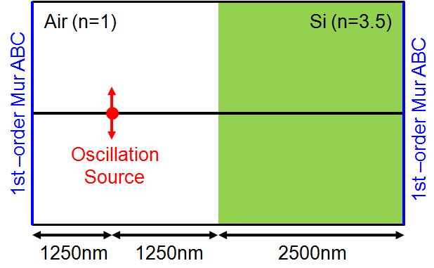
Example simulation is shown in Fig. 1. The computational domain is 5000nm.
The wave generated by a point source propagates in air and silicon media.
The computational domain is terminated by the first-order Mur absorbing boundary condition (ABC).
Fig. 1. Example simulation. Computational domain is 5000nm. The left side of computational domain consists of air and the right side is silicon (n = refractive index).
The both sides are terminated by the first-order Mur absorbing boundary condition. An oscillation source is at a grid point.
Simulation parameters are listed in Table 1. The wavelength λ = 1550nm is widely used in optical communication.
The grid spacing Δx is 50nm, considering that one wavelength should be represent by 10 or more grid points to accurately calculate its propagation.
Table. 1. Simulation parameters.
| Source wavelength λ |
Grid spaceing Δx |
| 1550nm |
50nm |
Let us program the FDTD simulation using C++ language.
We first describe the FDTD computaion class, and next present its visualized demonstration using OpenGL.
FDTD Computation
We describe the one-dimensional FDTD simulation class in Source 1.
This is the standard FDTD program, but it can be expand to the nonstandard version by replacing uS with uNS.
Source 1. One-dimensional FDTD calculation class. [Download Source 1]
class FDTD1D {
private:
    // constants
    int    num;      // number of grid points
    double v;        // wave speed
    double dx;       // grid spacing
    double dt;       // time interval
    double lambda;   // wavelength
    double k;        // wavenumber
    double omega;    // angular frequency
    double n;        // refractive index
    // variables
    double* psi_next;       // next field
    double* psi_current;    // current field
    double* psi_previous;   // previous field
    double* u;              // coefficient matrix
    double  t;              // simulation time

public:
    // Initialization
    void Initialize( void )
    {
        num    = 100;             // number of grid points
        dx     =   1;             // grid spacing
        dt     =   1;             // time interval
        v      =   dx /  dt;      // wave speed
        lambda = 1550 /  50;      // wavelength
        k      = 2*M_PI/lambda;   // wavenumber
        omega  =    v *   k;      // angular frequency
        n      = 3.5;             // refractive index

        // Get memory
        psi_next     = new double [num];
        psi_current  = new double [num];
        psi_previous = new double [num];
        u            = new double [num];

        // Set init field
        for ( int i=0; i<num; i++ ) {
            // wave field
            psi_next[i] = psi_current[i] = psi_previous[i] = 0;
            // media distribution
            if ( i < num/2 ) u[i] =   v * dt/dx;
            else             u[i] = v/n * dt/dx;
        }
    }

    // Finalize
    void Finalize( void )
    {
        // Release memory
        delete [] psi_next;
        delete [] psi_current;
        delete [] psi_previous;
        delete [] u;
    }

    // Absorbing boundary condition (ABC)
    void MurABC( void )
    {
        // Left boundary
        psi_next[0] = psi_current[1]
            + (u[0]-1)/(u[0]+1) * (psi_next[1] - psi_current[0]);
        // Right boundary
        psi_next[num-1] = psi_current[num-2]
            + (u[num-1]-1)/(u[num-1]+1)
            * (psi_next[num-2] - psi_current[num-1]);
    }

    // Update field
    void Update( void )
    {
        // Shift memory target
        double* temp = psi_previous;
        psi_previous = psi_current;
        psi_current  = psi_next;
        psi_next     = temp;

        // Update field
        for ( int i=1; i<num-1; i++ ) {
            // Update each grid point
            psi_next[i] = - psi_previous[i] + 2*psi_current[i]
                + u[i]*u[i]
                * (psi_current[i+1]-2*psi_current[i]+psi_current[i-1]);
            // Add source
            if ( i == num/4 ) psi_next[i] = sin( omega*t );
        }

        // Set absorbing boundary condition
        MurABC();

        // Update t
        t += dt;
    }

    // Get number of grid points
    int GetNum()
    {
        return num;
    }

    // Get next field value
    double GetValue( int idx )
    {
        return psi_next[idx];
    }
};
|
The functions are
- Initialize:
(1) Define simulation parameters; (2) Allocate field and coefficient memoris; (3) Initialize field and set media distribution.
- Finalize:
Release memories.
- MurABC:
Set the first-order Mur ABC at (1) left side boundary; (2) right side boundary.
- Update:
Calculate next time step. (1) Shift memory target; (2) Update field using the FDTD algorithm. The oscillation source is given at num/4; (3) Set Mur ABC; (4) Update time step.
- GetNum:
Return the number of grid points.
- GetValue:
Return calculated field value indexed by idx.
We can simulate wave propagation in Fig. 1 using Source 1, but a visualization is necessary to validate the calculated result.
Next, we introduce a simple visualization using OpenGL.
OpenGL Visualization
OpenGL is an powerful application program interface, but its parameters are much complicated.
Instead the OpenGL utility toolkit (GLUT) provides simple procedure of the OpenGL controls.
The GLUT can be obtained at
Let us program an interactive calculation using the GLUT.
Source 2 is a main program includes GLUT visualization.
Source 2. GLUT visualization of FDTD simulation. [Download Source 2]
// Include header files
#include "fdtd1d.h"
#include "glut.h"

// FDTD1D class
FDTD1D fdtd;

// Keyboard event
void keyboard( unsigned char key, int x, int y )
{
    switch ( key ) {
        // pushed 't' key
        case 't':
            fdtd.Update();         // Update field
            glutPostRedisplay();   // Redisplay
            break;
        default:
            break;
    }
}

// Redisplay event
void display( void )
{
    // Clear background
    glClear( GL_COLOR_BUFFER_BIT );

    // Set line width
    glLineWidth( 3 );
    // Set line color
    glColor3d( 1, 1, 1 );
    // Draw continuous line (canvas is x = -1...+1, y = -1...+1)
    glBegin( GL_LINE_STRIP );
        for ( int i=1; i<fdtd.GetNum()-1; i++ ) {
            double x = 2*i/(fdtd.GetNum()-1.0) - 1;
            double y = fdtd.GetValue(i);
            glVertex2d( x, y );
        }
    glEnd();

    // Update view
    glFlush();
}

// Main function
int main( int argc, char** argv )
{
    // Initialize OpenGL
    glutInitWindowPosition( 100, 100 );   // window position
    glutInitWindowSize( 640, 480 );       // window size
    glutInitDisplayMode( GLUT_SINGLE );   // display mode
    glutInit( &argc, argv );              // Initialize GLUT
    glutCreateWindow( "FDTD" );           // Create window
    glutKeyboardFunc( keyboard );         // Register keyboard events
    glutDisplayFunc( display );           // Register display events

    // Initialize
    fdtd.Initialize();

    // GL loop
    glutMainLoop();

    // Finalize
    fdtd.Finalize();

    return 0;
}
|
We recommend studying the GLUT in many web sites introduce details.
Here we show rough flow of functions,
- keyboard:
Reply to keyboard events, where for t-key: (1) Update wave field; (2) Post a display event.
- display:
Draw figures: (1) Clear canvas; (2) Draw continuous line corresponded to wave field; (3) Display the figure.
- main:
(1) Initialize OpenGL using GLUT library; (2) Initialize FDTD class; (3) Start main loop. This loop is held up processing events until the window is closed; (4) Finalize FDTD class.
Figure 2 show the FDTD simulation result of Source 2. The monochromatic wave generated at point source propagate to both sides.
A part of the wave is reflected at the medium interface between air and silicon. There is no reflection at Mur ABCs.
Fig. 2. FDTD simulation result.
Copyright (C) 2011 Naoki Okada, All Rights Reserved.