Nonstandard FDTD Theory

Beginner Course

1. Finite Difference Model
2. 1D Wave Equation
3. 1D Stability
4. 1D Boundary Condition
5. Dimensionless Form
6. 1D Example

Intermediate Course

1. 2D Wave Equation
2. 2D Maxwell's Equations
3. Scattered Field
4. 2D Stability
5. 2D Boundary Condition
6. Scatterer Representation
7. Intensity
8. 2D Example

Advanced Course

1. 3D Wave Equation
2. 3D Maxwell's Equations
3. 3D Stability
4. Conductive Media
5. Perfectly Matched Layer

6. Scatterer Representation

A high-accuracy FDTD algorithm alone does not always guarantee a high-accuracy result, because other errors enter into the total calculation such as how the computational boundaries are terminated and how the scatterers are modeled on the numerical grid. The boundary error can be reduced very small by good absorbing boundary conditions such as the perfectly matched layer, so the largest remaining source of error is the representation of the scatterer. We introduce the simple method called staircase model and high accuracy one called fuzzy model.

Staircase Model

The most elementary representation is the staircase model. A grid point is either inside or outside the scatterer. In Fig. 1(a), a scatterer of permittivity ε₁ (gray region) is immersed in a medium of permittivity ε₂ (white region). In the staircase model ε(r) = ε₁ if grid point r lies within the scatterer (A and C), and ε(r) = ε₂ otherwise (B and D).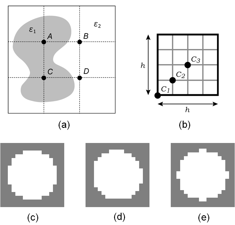

Fig. 1. Staircase model. (a) Example grid points. A and C are inside scatterer (gray), B and D are outside (white). (b) circle center C₁ is on a grid point, C₃ is centered in a cell, C₂ lies between C₁ and C₃. (c), (d), (e) are circle models centered at C₁, C₂, C₃, respectively.

However, the staircase model obviously cannot include distributions between grid points, and fails to accurately model the shape. For example, consider the circles centered at C₁, C₂, and C₃ on a uniform grid of spacing h and their corresponding staircase representation in Fig. 1(b). As shown in Figs. 1(c), (d), (e), the representations are various with the position of circle center and indicate increasing the representation error.

Fuzzy Model

The fuzzy model is much better than the staircase model, because the scatterer shape are accurately represented. The fuzzy model is derived from Ampere's law,

First let us consider in the TM mode. Extracting the E_z component from the left side of (1), we evaluate the integral over the surface shown in Fig. 2(a).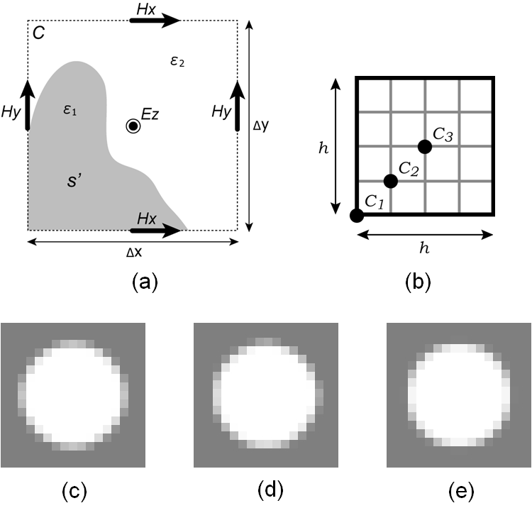

Fig. 2. Fuzzy model in the TM mode. (a) Integration of H on contour about E_z grid point. (b) circle center C₁ is on a grid point, C₃ is centered in a cell, C₂ lies between C₁ and C₃. (c), (d), (e) are circle models centered at C₁, C₂, C₃, respectively.

If Δx and Δy are sufficiently small, we find

Similarly H is essentially constant in Fig. 2(a). Using Stoke's theorem, the right side of (1) becomes

On the other hand, since ε must be a constant at a grid point in FDTD calculations, the differential form of Ampere's law is given by

where <ε>_xy means the average of ε on the x-y surface about the grid point. Comparing (4) with (2) and (3), we obtain

The fuzzy model assures a continuous range of values between ε₁ and ε₂ on the calculation grid, rather than the binary values of the staircase model. When the cylinder center is shifted in Fig 2(b), the symmetries are better presented than the staircase model as shown in Fig. 2(c), (d), (e).

In the TE mode, the fuzzy model is derived by integrating E_x on the y-z plane and E_y on the x-z plane. Because the scatterer distributions are constant in the z-direction, ε is replaced by line averages. For example, as shown in Fig. 3(a), E_x lies at r = (x, y+Δy/2).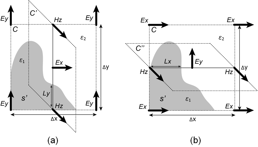

Fig. 3. The fuzzy model in the TE mode. (a) Integration of H on contour about E_x grid point. (b) Integration of H on contour about E_y grid point.

Here ε(r) on the x-y surface is replaced by

Similarly, as shown in Fig. 3(b), E_y lies at r = (x+Δx/2, y) and ε(r) is replaced by

In three dimensions, the fuzzy model is the same as the formulation in the TE mode, because E_x, E_y, E_z are obtained by integration on the y-z, x-z, x-y surfaces, respectively.

Copyright (C) 2011 Naoki Okada, All Rights Reserved.