Nonstandard FDTD Theory

Beginner Course

1. Finite Difference Model
2. 1D Wave Equation
3. 1D Stability
4. 1D Boundary Condition
5. Dimensionless Form
6. 1D Example

Intermediate Course

1. 2D Wave Equation
2. 2D Maxwell's Equations
3. Scattered Field
4. 2D Stability
5. 2D Boundary Condition
6. Scatterer Representation
7. Intensity
8. 2D Example

Advanced Course

1. 3D Wave Equation
2. 3D Maxwell's Equations
3. 3D Stability
4. Conductive Media
5. Perfectly Matched Layer

5. Dimensionless Form

In electromagnetic simulations, uses of physical parameters cause instability. For example, if physical parameters are used (program codes involve Δx = 0.00000001, Δt = 0.00000000000000003, v = 300000000) as shown in Table 1, our double-precision floating point operators increase loss of trailing digits and fail the calculation.

Table. 1. Example physical parameters.

Grid spaceing Δx	Time interval Δt	Light speed v
10 nm	0.03 fs	3 × 108 m/s

Instead we define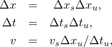

where Δx_s, Δt_s, v_s are non-dimensional parameters, and Δx_u, Δt_u are unit quantities. Given Δx, Δt, and v, we can freely choose Δx_s, Δt_s, v_s under the numerical stability adjusting Δx_u and Δt_u. Let us transform the one-dimensional wave equation to dimenshonless form. The wave equation is given by

Substituting (1) into (2), we obtain

Thus we can solve the same equation without using physical parameters. For simplicity, we always use Δx_s = Δt_s = 1.

Example Parameter Setting

Let us consider that a monochromatic wave of wavelength λ = 1500nm. Let Δx = 10nm and Δx_s = Δt_s = 1. The numerical stability is given by

The dimensionless wavelength becomes

and the dimensionless wave period becomes

Thus the monochromatic wave in dimensionless form is given by

Copyright (C) 2011 Naoki Okada, All Rights Reserved.